August | 2011

The smoothed UKF performs smoothing on the state system a-posteriori. The standard form of this filter is useful in getting an accurate view on prior states, but will not provide a smoothed online state estimate for the current or next period (i.e. no better estimate than the non-smoothed UKF).

That said the smoothed UKF is still useful as:

can be used to estimate the MLE for a stable parameter
a timeseries of smoothed prior states can be regressed to project a smoothed forward state (but is not part of the UKF framework)

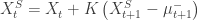
The form of UKF smoother that will briefly discuss is the forward-backward smoother. As the name suggests, the first pass is to perform standard UKF filter, estimating the distribution $p({x_t}|{x_{t - 1}},{y_{1:t}})$ at each timestep. Whereas the smoothing estimates a smoothed distribution in reverse, implying $p(x_{t - 1}^S|x_t^S,\Sigma _t^S)$ . The boundary $x_T^S,\Sigma _T^S$ is simply the last state and covariance estimated by the forward filter.

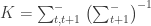
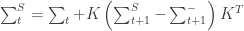
The smoothing approach is then for each $x_{t }^S, \Sigma _t^S$ , determine the predicted $x_{t+1 }^-, \Sigma _{t+1}^-, \Sigma _{t,t+1}^-$ , and back out an appropriate adjustment given a computed kalman gain and the difference between the predicted t+1 and actual t+1 state:

$\left[\mu _{t+1}^ - ,\sum _{t+1}^ - ,\sum _{t,t + 1}^ - \right] = UT\left( {{X_t},\sum _{t,t}^{},f(.), \cdots } \right)$

$K = \sum _{t,t + 1}^ - {\left( {\sum _{t + 1}^ - } \right)^{ - 1}}$
$X_t^S = X_t^{} + K\left( {X_{t + 1}^S - \mu _{t + 1}^ - } \right)$
$\sum _t^S = \sum _t^{} + K\left( {\sum _{t + 1}^S - \sum _{t + 1}^ - } \right){K^T}$

Results
A simple example of a non-linear function is the Sine function. Tracking the sine function using a linearization of the sine function with standard Kalman filter will perform poorly. My test case for the UKF was the following function with noise:

$y(t) = {a_t}\sin \left( {{\theta _t}} \right) + {\varepsilon _t}$

where ${a_t}$ and $\theta _t$ are linear functions of time. The states in the system track: $A(t),\frac{{dA}}{{dt}},\theta (t),\frac{{d\theta }}{{dt}}$ . Here is UKF tracking without smoothing:

And here is the same with smoothing:

Code
I’m enclosing R code for the augmented UKF and smoothed UKF. For readability I have not optimized all of the R code (i.e. there are some for loops that could be vectorized). Here is the common part (defining the Unscented Transform).

## modified number of columns
ncols <- function (x) ifselse(is.matrix(x), ncol(x), length(x))

## modified number of rows
nrows <- function (x) ifelse(is.matrix(x), nrow(x), length(x))

#
#	Determine transformed distribution across non-linear function f(x)
#
#
unscented.transform.aug <- function (
	MUx,				# mean of state
	P, 					# covariance of state
	Nyy,				# noise covariance matrix of f(x)
	f,					# non-linear function f(X, E)
	dt,					# time increment
	alpha = 1e-3,		# scaling of points from mean
	beta = 2,			# distribution parameter
	kappa = 1)
{
	Nyy <- as.matrix(Nyy)

	## constants
	Lx <- nrows(MUx)
	Ly <- nrows(Nyy)
	n <- Lx + Ly

	## create augmented mean and covariance
	MUx.aug <- c (MUx, rep(0, Ly))
	P.aug <- matrix(0, Lx+Ly, Lx+Ly)
	P.aug[1:Lx,1:Lx] <- P
	P.aug[(Lx+1):(Lx+Ly),(Lx+1):(Ly+Ly)] <- Nyy

	## generating sigma points
	lambda <- alpha^2 * (n + kappa) - n
	A <- t (chol (P.aug))
	X <- MUx.aug + sqrt(n + lambda) * cbind (rep(0,n), A, -A)

	## generate weights
	Wc <- c (
		lambda / (n + lambda) + (1 - alpha^2 + beta),
		rep (1 / (2 * (n + lambda)), 2*n))
	Wm <- c (
		lambda / (n + lambda),
		rep (1 / (2 * (n + lambda)), 2*n))

	## propagate through function
	Y <- apply(X, 2, function (v)
		{
			f (dt, v[1:Lx], v[(Lx+1):(Lx+Ly)])
		})

	if (is.vector(Y))
		Y <- t(as.matrix(Y))

	## now calculate moments
	MUy <- Y %*% Wm

	Pyy <- matrix(0, nrows(Nyy), nrows(Nyy))
	Pxy <- matrix(0, nrows(MUx), nrows(Nyy))

	for (i in 1:ncols(Y))
	{
		dy <- (Y[,i] - MUy)
		dx <- (X[1:Lx,i] - MUx)

		Pyy <- Pyy + Wc[i] * dy %*% t(dy)
		Pxy <- Pxy + Wc[i] * dx %*% t(dy)
	}

	list (mu = MUy, Pyy = Pyy, Pxy = Pxy)
}

The UKF without smoothing:

#
#	Augmented UKF filtered series
#		- note that f and g are functions of state X and error vector N  f(dt, Xt, E)
#		- Nx and Ny state and observation innovation covariance
#		- Xo is the initial state
#		- dt is the time step
#
ukf.aug <- function (
	series,
	f,
	g,
	Nx,
	Ny,
	Xo = rep(0, nrow(Nx)),
	dt = 1,
	alpha = 1e-3,
	kappa = 1,
	beta = 2)
{
	data <- as.matrix(coredata(series))

	## description of initial distribution of X
	oMUx <- Xo
	oPx <- diag(rep(1e-4, nrows(Xo)))

	Yhat <- NULL
	Xhat <- NULL

	for (i in 1:nrow(data))
	{
		Yt <- t(data[i,])

		## predict
		r <- unscented.transform.aug (oMUx, oPx, Nx, f, dt, alpha=alpha, beta=beta, kappa=kappa)
		pMUx <- r$mu
		pPx <- r$Pyy

		## update
		r <- unscented.transform.aug (pMUx, pPx, Ny, g, dt, alpha=alpha, beta=beta, kappa=kappa)
		MUy <- r$mu
		Pyy <- r$Pyy
		Pxy <- r$Pxy

		K <- Pxy %*% inv(Pyy)
		MUx = pMUx + K %*% (Yt - MUy)
		Px <- pPx - K %*% Pyy %*% t(K)

		## set for next cycle
		oMUx <- MUx
		oPx <- Px

		## append results
		Yhat <- rbind(Yhat, t(MUy))
		Xhat <- rbind(Xhat, t(MUx))
	}

	list (Yhat = Yhat, Xhat = Xhat)
}

The UKF with smoothing:

ukf.smooth <- function (
	series, 					# series to be filtered
	f, 							# state mapping X[t] = f(X[t-1])
	g, 							# state to measure mapping Y[t] = g(X[t])
	Nx, 						# state innovation error covar
	Ny, 						# measure innovation covar
	Xo = rep(0, nrow(Nx)), 		# initial state vector
	dt = 1, 					# time increment
	alpha = 1e-3,
	kappa = 1,
	beta = 2)
{
	data <- as.matrix(coredata(series))

	Lx <- nrow(as.matrix(Nx))
	Ly <- nrow(as.matrix(Ny))

	## description of initial distribution of X
	oMUx <- Xo
	oPx <- diag(rep(1e-4, nrows(Xo)))

	Ey <- rep(0, nrows(Ny))
	Ex <- rep(0, nrows(Nx))

	Ms <- list()
	Ps <- list()

	## forward filtering
	for (i in 1:nrow(data))
	{
		Yt <- t(data[i,])

		## predict
		r <- unscented.transform.aug (oMUx, oPx, Nx, f, dt, alpha=alpha, beta=beta, kappa=kappa)
		pMUx <- r$mu
		pPx <- r$Pyy

		## update
		r <- unscented.transform.aug (pMUx, pPx, Ny, g, dt, alpha=alpha, beta=beta, kappa=kappa)
		MUy <- r$mu
		Pyy <- r$Pyy
		Pxy <- r$Pxy

		K <- Pxy %*% inv(Pyy)
		MUx = pMUx + K %*% (Yt - MUy)
		Px <- pPx - K %*% Pyy %*% t(K)

		## set for next cycle
		oMUx <- MUx
		oPx <- Px

		## append results
		Ms[[i]] <- MUx
		Ps[[i]] <- Px
	}

	## backward filtering, recursively determine N(Ms[t-1],Ps[t-1]) from N(Ms[t],Ps[t])
	for (i in rev(1:(nrow(data)-1)))
	{
		## transform
		r <- unscented.transform.aug (Ms[[i]], Ps[[i]], Nx, f, dt, alpha=alpha, beta=beta, kappa=kappa)
		MUx <- r$mu
		Pxx <- r$Pyy
		Pxy <- r$Pxy[1:Lx,]

		K <- Pxy %*% inv(Pxx)
		Ms[[i]] <-  Ms[[i]] + K %*% (Ms[[i+1]] - MUx)
		Ps[[i]] <- Ps[[i]] + K %*% (Ps[[i+1]] - Pxx) * t(K)
	}

	Yhat <- NULL
	Xhat <- NULL

	for (i in 1:nrow(data))
	{
		MUy <- g(dt, Ms[[i]], Ey)
		MUx <- Ms[[i]]

		## append results
		Yhat <- rbind(Yhat, t(MUy))
		Xhat <- rbind(Xhat, t(MUx))
	}

	list (Y = data, Yhat = Yhat, Xhat = Xhat)
}

Finally, here is the Sine test:

#
#	Amplitude varying sine function state function:
#
#		Yt = Amp[t] Sin(theta[t]) + Ey
#
#		Theta[t] = Theta[t-1] + Omega[t-1] dt + Ex,1
#		Omega[t] = Omega[t-1] + Ex,2
#		Amp[t] = Amp[t-1] + Accel[t-1] dt + Ex,3
#		Accel[t] = Accel[t] + Ex,4
#
sine.f.xx <- function (dt, Xt, Ex)
{
	nXt <- c (
		Xt[1] + dt*Xt[2] + Ex[1],
		Xt[2] + Ex[2],
		Xt[3] + Ex[3],
		Xt[4] + Ex[4])

	nXt
}

#
#	Amplitude varying sine function observation function:
#
#		Yt = Amp[t] Sin(theta[t]) + Ey
#
#		Theta[t] = Theta[t-1] + Omega[t-1] dt + Ex,1
#		Omega[t] = Omega[t-1] + Ex,2
#		Amp[t] = Amp[t-1] + Accel[t-1] dt + Ex,3
#		Accel[t] = Accel[t] + Ex,4
#
sine.f.xy <- function (dt, Xt, Ey)
{
	y <- Xt[3] * sin(Xt[1] / pi) + Ey[1]
	as.matrix(y)
}

#debug(unscented.transform.aug)
#debug(ukf.aug)

series.r <- sapply (1:500, function(x) (1+x/500) * sin(16 * x/500 * pi)) + rnorm(500, sd=0.25)

## unsmoothed test
u <- ukf.aug (
	series.r, sine.f.xx, sine.f.xy,
	Nx = 1e-3 * diag(c(1/3, 1, 1/10, 1/10)),
	Ny = 1,
	Xo = c(0.10, 0.10, 1, 1e-3), alpha=1e-2)

data <- rbind (
	data.frame(t = 1:500, y=series.r, type='raw', window='Price'),
	data.frame(t = 1:500, y=u$Yhat, type='filtered', window='Price'),
	data.frame(t = 1:500, y=u$Xhat[,3], type='amp', window='Params'))

ggplot() + geom_line(aes(x=t,y=y, colour=type), data) + facet_new(window ~ ., scales="free_y", heights=c(3,1))

## smoothed test
u <- ukf.smooth (
	series.r, sine.f.xx, sine.f.xy,
	Nx = 1e-3 * diag(c(1/3, 1, 1/10, 1/10)),
	Ny = 1,
	Xo = c(0.10, 0.10, 1, 1e-3), alpha=1e-2)

data <- rbind (
	data.frame(t = 1:500, y=series.r, type='raw', window='Price'),
	data.frame(t = 1:500, y=u$Yhat, type='filtered', window='Price'),
	data.frame(t = 1:500, y=u$Xhat[,3], type='amp', window='Params'))

ggplot() + geom_line(aes(x=t,y=y, colour=type), data) + facet_new(window ~ ., scales="free_y", heights=c(3,2))

If you find the above code useful or have improvements to suggest, kindly send me a note. Thanks.

Next Steps
Some next steps:

Determine state-system appropriate for market making & cycling regimes
Determine Multi-Model switching approach
Evaluation & Analysis

I will probably make a digression onto another topic in the next posting before revisiting this. Stay tuned.

p.s. if you use wordpress, they have a latex equation rendering capability I just discovered (hence better inlining in this post).

Monthly Archives: August 2011

Smoothed UKF

Search

Recent Entries

Links

Bitcoin

Resources

Strategy