The smoothed UKF performs smoothing on the state system a-posteriori. The standard form of this filter is useful in getting an accurate view on prior states, but will not provide a smoothed online state estimate for the current or next period (i.e. no better estimate than the non-smoothed UKF).
That said the smoothed UKF is still useful as:
- can be used to estimate the MLE for a stable parameter
- a timeseries of smoothed prior states can be regressed to project a smoothed forward state (but is not part of the UKF framework)
The form of UKF smoother that will briefly discuss is the forward-backward smoother. As the name suggests, the first pass is to perform standard UKF filter, estimating the distribution 


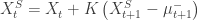
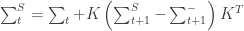
The smoothing approach is then for each 

![\left[\mu _{t+1}^ - ,\sum _{t+1}^ - ,\sum _{t,t + 1}^ - \right] = UT\left( {{X_t},\sum _{t,t}^{},f(.), \cdots } \right)](https://s0.wp.com/latex.php?latex=%5Cleft%5B%5Cmu+_%7Bt%2B1%7D%5E+-+%2C%5Csum+_%7Bt%2B1%7D%5E+-+%2C%5Csum+_%7Bt%2Ct+%2B+1%7D%5E+-+%5Cright%5D+%3D+UT%5Cleft%28+%7B%7BX_t%7D%2C%5Csum+_%7Bt%2Ct%7D%5E%7B%7D%2Cf%28.%29%2C+%5Ccdots+%7D+%5Cright%29&bg=ffffff&fg=333333&s=0&c=20201002)
Results
A simple example of a non-linear function is the Sine function. Tracking the sine function using a linearization of the sine function with standard Kalman filter will perform poorly. My test case for the UKF was the following function with noise:

where 


And here is the same with smoothing:

Code
I’m enclosing R code for the augmented UKF and smoothed UKF. For readability I have not optimized all of the R code (i.e. there are some for loops that could be vectorized). Here is the common part (defining the Unscented Transform).
## modified number of columns
ncols <- function (x) ifselse(is.matrix(x), ncol(x), length(x))

## modified number of rows
nrows <- function (x) ifelse(is.matrix(x), nrow(x), length(x))

#
#	Determine transformed distribution across non-linear function f(x)
#
#
unscented.transform.aug <- function (
	MUx,				# mean of state
	P, 					# covariance of state
	Nyy,				# noise covariance matrix of f(x)
	f,					# non-linear function f(X, E)
	dt,					# time increment
	alpha = 1e-3,		# scaling of points from mean
	beta = 2,			# distribution parameter
	kappa = 1)
{
	Nyy <- as.matrix(Nyy)

	## constants
	Lx <- nrows(MUx)
	Ly <- nrows(Nyy)
	n <- Lx + Ly

	## create augmented mean and covariance
	MUx.aug <- c (MUx, rep(0, Ly))
	P.aug <- matrix(0, Lx+Ly, Lx+Ly)
	P.aug[1:Lx,1:Lx] <- P
	P.aug[(Lx+1):(Lx+Ly),(Lx+1):(Ly+Ly)] <- Nyy

	## generating sigma points
	lambda <- alpha^2 * (n + kappa) - n
	A <- t (chol (P.aug))
	X <- MUx.aug + sqrt(n + lambda) * cbind (rep(0,n), A, -A)

	## generate weights
	Wc <- c (
		lambda / (n + lambda) + (1 - alpha^2 + beta),
		rep (1 / (2 * (n + lambda)), 2*n))
	Wm <- c (
		lambda / (n + lambda),
		rep (1 / (2 * (n + lambda)), 2*n))

	## propagate through function
	Y <- apply(X, 2, function (v)
		{
			f (dt, v[1:Lx], v[(Lx+1):(Lx+Ly)])
		})

	if (is.vector(Y))
		Y <- t(as.matrix(Y))

	## now calculate moments
	MUy <- Y %*% Wm

	Pyy <- matrix(0, nrows(Nyy), nrows(Nyy))
	Pxy <- matrix(0, nrows(MUx), nrows(Nyy))

	for (i in 1:ncols(Y))
	{
		dy <- (Y[,i] - MUy)
		dx <- (X[1:Lx,i] - MUx)

		Pyy <- Pyy + Wc[i] * dy %*% t(dy)
		Pxy <- Pxy + Wc[i] * dx %*% t(dy)
	}

	list (mu = MUy, Pyy = Pyy, Pxy = Pxy)
}
The UKF without smoothing:
#
# Augmented UKF filtered series
# - note that f and g are functions of state X and error vector N f(dt, Xt, E)
# - Nx and Ny state and observation innovation covariance
# - Xo is the initial state
# - dt is the time step
#
ukf.aug <- function (
series,
f,
g,
Nx,
Ny,
Xo = rep(0, nrow(Nx)),
dt = 1,
alpha = 1e-3,
kappa = 1,
beta = 2)
{
data <- as.matrix(coredata(series))
## description of initial distribution of X
oMUx <- Xo
oPx <- diag(rep(1e-4, nrows(Xo)))
Yhat <- NULL
Xhat <- NULL
for (i in 1:nrow(data))
{
Yt <- t(data[i,])
## predict
r <- unscented.transform.aug (oMUx, oPx, Nx, f, dt, alpha=alpha, beta=beta, kappa=kappa)
pMUx <- r$mu
pPx <- r$Pyy
## update
r <- unscented.transform.aug (pMUx, pPx, Ny, g, dt, alpha=alpha, beta=beta, kappa=kappa)
MUy <- r$mu
Pyy <- r$Pyy
Pxy <- r$Pxy
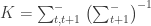
K <- Pxy %*% inv(Pyy)
MUx = pMUx + K %*% (Yt - MUy)
Px <- pPx - K %*% Pyy %*% t(K)
## set for next cycle
oMUx <- MUx
oPx <- Px
## append results
Yhat <- rbind(Yhat, t(MUy))
Xhat <- rbind(Xhat, t(MUx))
}
list (Yhat = Yhat, Xhat = Xhat)
}
The UKF with smoothing:
ukf.smooth <- function (
	series, 					# series to be filtered
	f, 							# state mapping X[t] = f(X[t-1])
	g, 							# state to measure mapping Y[t] = g(X[t])
	Nx, 						# state innovation error covar
	Ny, 						# measure innovation covar
	Xo = rep(0, nrow(Nx)), 		# initial state vector
	dt = 1, 					# time increment
	alpha = 1e-3,
	kappa = 1,
	beta = 2)
{
	data <- as.matrix(coredata(series))

	Lx <- nrow(as.matrix(Nx))
	Ly <- nrow(as.matrix(Ny))

	## description of initial distribution of X
	oMUx <- Xo
	oPx <- diag(rep(1e-4, nrows(Xo)))

	Ey <- rep(0, nrows(Ny))
	Ex <- rep(0, nrows(Nx))

	Ms <- list()
	Ps <- list()

	## forward filtering
	for (i in 1:nrow(data))
	{
		Yt <- t(data[i,])

		## predict
		r <- unscented.transform.aug (oMUx, oPx, Nx, f, dt, alpha=alpha, beta=beta, kappa=kappa)
		pMUx <- r$mu
		pPx <- r$Pyy

		## update
		r <- unscented.transform.aug (pMUx, pPx, Ny, g, dt, alpha=alpha, beta=beta, kappa=kappa)
		MUy <- r$mu
		Pyy <- r$Pyy
		Pxy <- r$Pxy

		K <- Pxy %*% inv(Pyy)
		MUx = pMUx + K %*% (Yt - MUy)
		Px <- pPx - K %*% Pyy %*% t(K)

		## set for next cycle
		oMUx <- MUx
		oPx <- Px

		## append results
		Ms[[i]] <- MUx
		Ps[[i]] <- Px
	}

	## backward filtering, recursively determine N(Ms[t-1],Ps[t-1]) from N(Ms[t],Ps[t])
	for (i in rev(1:(nrow(data)-1)))
	{
		## transform
		r <- unscented.transform.aug (Ms[[i]], Ps[[i]], Nx, f, dt, alpha=alpha, beta=beta, kappa=kappa)
		MUx <- r$mu
		Pxx <- r$Pyy
		Pxy <- r$Pxy[1:Lx,]

		K <- Pxy %*% inv(Pxx)
		Ms[[i]] <-  Ms[[i]] + K %*% (Ms[[i+1]] - MUx)
		Ps[[i]] <- Ps[[i]] + K %*% (Ps[[i+1]] - Pxx) * t(K)
	}

	Yhat <- NULL
	Xhat <- NULL

	for (i in 1:nrow(data))
	{
		MUy <- g(dt, Ms[[i]], Ey)
		MUx <- Ms[[i]]

		## append results
		Yhat <- rbind(Yhat, t(MUy))
		Xhat <- rbind(Xhat, t(MUx))
	}

	list (Y = data, Yhat = Yhat, Xhat = Xhat)
}
Finally, here is the Sine test:
#
#	Amplitude varying sine function state function:
#
#		Yt = Amp[t] Sin(theta[t]) + Ey
#
#		Theta[t] = Theta[t-1] + Omega[t-1] dt + Ex,1
#		Omega[t] = Omega[t-1] + Ex,2
#		Amp[t] = Amp[t-1] + Accel[t-1] dt + Ex,3
#		Accel[t] = Accel[t] + Ex,4
#
sine.f.xx <- function (dt, Xt, Ex)
{
	nXt <- c (
		Xt[1] + dt*Xt[2] + Ex[1],
		Xt[2] + Ex[2],
		Xt[3] + Ex[3],
		Xt[4] + Ex[4])

	nXt
}

#
#	Amplitude varying sine function observation function:
#
#		Yt = Amp[t] Sin(theta[t]) + Ey
#
#		Theta[t] = Theta[t-1] + Omega[t-1] dt + Ex,1
#		Omega[t] = Omega[t-1] + Ex,2
#		Amp[t] = Amp[t-1] + Accel[t-1] dt + Ex,3
#		Accel[t] = Accel[t] + Ex,4
#
sine.f.xy <- function (dt, Xt, Ey)
{
	y <- Xt[3] * sin(Xt[1] / pi) + Ey[1]
	as.matrix(y)
}

#debug(unscented.transform.aug)
#debug(ukf.aug)

series.r <- sapply (1:500, function(x) (1+x/500) * sin(16 * x/500 * pi)) + rnorm(500, sd=0.25)

## unsmoothed test
u <- ukf.aug (
	series.r, sine.f.xx, sine.f.xy,
	Nx = 1e-3 * diag(c(1/3, 1, 1/10, 1/10)),
	Ny = 1,
	Xo = c(0.10, 0.10, 1, 1e-3), alpha=1e-2)

data <- rbind (
	data.frame(t = 1:500, y=series.r, type='raw', window='Price'),
	data.frame(t = 1:500, y=u$Yhat, type='filtered', window='Price'),
	data.frame(t = 1:500, y=u$Xhat[,3], type='amp', window='Params'))

ggplot() + geom_line(aes(x=t,y=y, colour=type), data) + facet_new(window ~ ., scales="free_y", heights=c(3,1))

## smoothed test
u <- ukf.smooth (
	series.r, sine.f.xx, sine.f.xy,
	Nx = 1e-3 * diag(c(1/3, 1, 1/10, 1/10)),
	Ny = 1,
	Xo = c(0.10, 0.10, 1, 1e-3), alpha=1e-2)

data <- rbind (
	data.frame(t = 1:500, y=series.r, type='raw', window='Price'),
	data.frame(t = 1:500, y=u$Yhat, type='filtered', window='Price'),
	data.frame(t = 1:500, y=u$Xhat[,3], type='amp', window='Params'))

ggplot() + geom_line(aes(x=t,y=y, colour=type), data) + facet_new(window ~ ., scales="free_y", heights=c(3,2))
If you find the above code useful or have improvements to suggest, kindly send me a note. Thanks.
Next Steps
Some next steps:
- Determine state-system appropriate for market making & cycling regimes
- Determine Multi-Model switching approach
- Evaluation & Analysis
I will probably make a digression onto another topic in the next posting before revisiting this. Stay tuned.
p.s. if you use wordpress, they have a latex equation rendering capability I just discovered (hence better inlining in this post).

Dude, what are you doing if your number one objective is not estimating the next state? The game is forecasting, and you act as if the “online state estimate for the current or next period” is a secondary concern.
The filters do estimate the next state, however, with the smoothed backward-forward UKF only applies a-posteriori, and is not able to smooth the current state.
That information, however, is useful. In particular if you are looking for a MLE estimate of a stable parameter. In addition the smoothed priors can be used to project a function going forward a few timesteps using some regression on the prior smoothed states. This is generally superior to doing the same on unsmoothed states. It is not part of the smoothed UKF algorithm however.
>1.Determine state-system appropriate for market making & cycling regimes
IMHO, this is the most difficult part of a problem. Most markets after “normalizing” for volatility very hard to distinguish from random walk. And even if such “dynamic enifficiencies” exists, they are very fragmentar and lightweight in nature. And it seems very unlikely for me that it is possible to “cluster” them in some state-space (markovian) form.
However, using it for spreads(mean-reversion,etc), “yet another stochastic volatility model” or some multi-market model with dynamic cross-correlations… make more sense.
But it will be interesting to read if you find something. 🙂 And thanks for this, quite outstanding blog!
I generally agree with what you have said (aside from the random walk aspect). Yes, using SDEs on near-stationary processes (as one would have with spreads or appropriately weighted baskets) is a much easier task.
In my revisiting, did some exploration offline. One can certainly find SDEs that regress through price movements, however are hard to parameterize and may not have all of the attributes I am looking for. Will discuss in a few weeks. I will jump to another topic for a few weeks before returning to this.
to put my 5 cents in you research… you can cast tick flow in random walk form with something like this: tick[i – 1] > tick[i] -> +1, tick[i – 1] -1 , and then calculate +1,-1 runs. In general, “market making” regime wil be charecterized by temporal clustering of shorter runs and “trending” by longer.
Great to see real R code (and latex too!); nice complement to prose.
Just a quick note that your “modified” functions replicate the functionality of NROW() and NCOL(). Thanks for the great blog.
ah, I did not know that. Thanks for the tip.
I also find the automatic “recasting” of matrix to numeric annoying when matrices with single column or row are passed through certain functions.
Dear Sir,
Thanks for your very interesting post.
Is it possible to provide R code for an application of the UKF on a real example (eg DJI data series imported from a csv file: DJI.csv)
Thank you for your help.
Kind regards,
Adam Sotowicz
With a UKF one does not just apply data through it. One needs to design a system of equations that represent the dynamics of the system. The UKF can then estimate the changing parameters of the system that best fit the observed data (for instance the DJI). So the most important thing is to design your state system first.
Could you provide an example of a simple state transition that could be applied to DJI data.
What do you want to achieve? A state-space-model is used to estimate parameters (the state) of a system. One of the simplest usages would be to use to determine a smooth spline through data. You could also have some trend model, etc.
For an example of a spline using a linear system:
Y[t] = F X[t] + v[t]
X[t+1] = G X[t] + w[t]
Can define the mapping between the states X and observations Y, F as:
| 1 0 |
and the evolution of states G, as matrix:
| 1 1 |
| 0 1 |
Define the observation variance V as 1.0 and define the state covariance W as:
| 0 0 |
| 0 λ |
Where to get different degrees of smoothing try λ = 1e-5, 1e-8. The first will provide less smoothing and the second more.
I am interested in two aspects.
1. Smoothing, which I will attempt based on the example you provided.
2. Short term order flow prediction. Each data point/bar represents buy/sell pressure (between 0 and 100). I suppose this could fall under trend following. Would you be able to provide a simple model that makes use of trend following using the unscented filter.
Thank you for the response.
I would not try to model buy/sell pressure based on prices. You are really going to want to look at trade flow.
Yes it would definitely be based on trade flow. I have the model for determining the order flow imbalance (which is fairly simple and that is fine). The question is how does one incorporate such a metric into the UKF Kalman filter. My biggest disconnect in this is understanding how to take a an output series (eg. order flow imbalance values) and convert it into what is required to perform kalman on it. I’ve tried following http://becs.aalto.fi/en/research/bayes/ekfukf/documentation.pdf as well. Unfortunately it’s not straight forward (for me) on how to do this as the approach seems to change when moving from the linear to non linear versions of the filter.
Well, you don’t just apply “kalman” to data. As you know, you need to have a model that represents the transformation between the observations and the state you want to estimate. So the real question is not how to aply a kalman filter, but what state system accomplishes your denoising / information extraction goal.
The UKF does not do anything magcical, so if you get the “model” { F(x), G(x) } wrong, then the filter will perform poorly and not generate anything useful (I’ve been there).
With regard to buy/sell imbalance, you might be better off using a classifier, if your goal is to predict market direction / momentum. You could also look at point-processes, which are very relevant for this sort of event based data.
Can you please provide the inner workings of the “inv” function?
inv(m) just computes the inverse of a matrix.
I thought that I just didnt want to assume. In turn, the function should be “ginv” from the MASS package. Also I noticed a small error in relation to ggplot; facet_new should be facet_grid. However, I do wonder how the P.aug matrix (augmented covariance matrix) is ensured to always be at least positive semi-definite, can you explain?